At its core, PlotDevice is a set of graphics ‘commands’ that operate on a virtual ‘canvas’. Each of your scripts has its own private canvas which is created before the first line of code is executed. Some commands affect the canvas directly (such as those for setting its size() and background() color), while others allow you to add graphics objects at specific positions.

Drawing Basics

PlotDevice provides a set of commands for drawing text, images, and basic geometric shapes. Each of these drawing primitives takes a pair of x/y parameters to set its position. Based on the command-type this will be interpreted as either the top-left corner or a central ‘origin’ point. You’ll find yourself using both kinds of positioning depending on what you’re trying to accomplish.

Origin-based objects

Corner-based objects

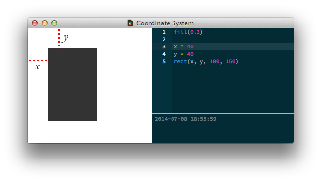
The coordinate system

When you place an element on the canvas, you define its position in terms of x and y coordinates. The ‘x’ is the horizontal position measured from the left of the canvas and the ‘y’ is the vertical position from the top.

PlotDevice has an ‘inverted’ coordinate system which might be confusing for those thinking back to their middle-school Algebra lessons. In a Cartesian coordinate system, moving a point lower on the graph means making its y value more negative. But in PlotDevice, downard movement means making y more positive.

We tend to prefer this scheme since page layouts tend to work relative to the top of the page rather than the bottom.

Syntax

In the Reference, each drawing primitive and its usage is discussed at length. The reference is something you’ll want to keep close at hand when you start learning PlotDevice. After a bit of experimentation you’ll know all the primitives by heart.

For example, take a look at documentation for the rect() command. As you might expect, this command draws a rectangle. At the top of the reference entry is a description of its syntax. The list of required and optional arguments provides the details you need to invoke the command in a way that PlotDevice understands.

In the rect() command’s case, the syntax is:

rect(x, y, width, height, roundness=0.0, plot=True)

All commands in PlotDevice look like this: you have the name of the command (rect for example) which gives you a hint of what the command will do, and some stuff between parentheses. The items within the ‘parens’ will be referred to as parameters or arguments interchangeably.

Parameters

A ‘rectangle’ could be a number of different things. For instance, a rectangle with an equal width and height would be a ‘square’. We could conceivably have another command called square() to draw them. Or imagine another rectangle that’s small and positioned at the bottom of the canvas. We could have a command for that called smallbottomrect(). The list goes on … we could define an infinite number of commands for rectangles of all shapes and sizes!

But instead of this multitude of commands, PlotDevice provides just a single rect() command that uses parameters to handle these different scenarios. Parameters are values you can customize to change the command’s behavior. You can supply numbers, variables, strings, or even objects as parameters depending on what the command knows how to handle.

For example, to draw a square at the canvas’s origin in the top left corner with a size of 40 we’d use parameters like:

rect(0, 0, 40, 40)

Notice how we replaced the x, y, width and height from the syntax description with real numbers. These number parameters describe how our rectangle will look: it is positioned at the top (y is 0) left (x is 0) edge of the canvas and has an equal width and height of 40.

Optional parameters

You’ll notice some other parameters in the rect() syntax which we didn’t define, the roundness=0.0 for example. If a parameter description has an =something next to it, this means it is optional. If we don’t define this parameter in our script, it’s default value is something. In the rectangle command’s case the corner roundness defaults to zero unless we explicitly say:

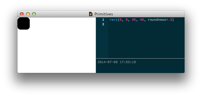
rect(0, 0, 40, 40, roundness=0.5)

Now we have a rectangle with 50% round corners:

The ‘plot’ parameter

All of the primitives have an optional argument called plot which defaults to True. This is a hint that just by calling the command you’ll be adding a new shape to the canvas. In general this is exactly what you intended, but there are certain special cases where you’ll want to store a not-yet-drawn primitive in a variable for use later on.

You can accomplish this by calling the command with an optional argument of plot=False. When you’re ready to add the primitive to the canvas, call the plot() command with the reference you saved as its sole parameter:

square = rect(50,50, 100,100, plot=False) # don't draw yet
... # do other things
plot(square) # add the square to the canvas

Defining your own shape-drawing commands

It’s not that difficult to create your own commands in PlotDevice. In the Commands tutorial you’ll learn how to create a function that combines calls to the basic shapes to create more-intricate graphics. Also look at the tutorial on Béziers to see how you can draw freeform shapes of your choosing.