More often than not, your PlotDevice scripts will involve at least a bit of mathematics. Things like fluid motion, orbital behavior, and easing-in and -out all require a little number-crunching. But fear not, this chapter collects some of the more-useful math tools for dealing with 2D drawing.
Transformation State
When you draw primitives to the PlotDevice canvas, their position is specified relative to the ‘origin’ in the upper left corner. By changing the ‘transformation state’, you can modifiy the location of the origin point which will affect how all subsequent pairs of coordinates are translated into canvas positions.
Perhaps it’s easiest to think of transformation state in terms of a real-world pen & paper analogy. When you move the pen to a pair of coordinates, your arm moves a relative distance from its starting point. When you change transformation state, you’re picking up the pen and shifting the paper before making the same arm movements as before.
Basic transformations
To get a sense of how transformations interact with drawing commands, let’s look at the translate() command. It allows you to shift the canvas horizontally and vertically (but without changing its orientation or size). For instance, when you say:
rect(20, 40, 80, 80)
a rectangle with a width and a height of 80 will be positioned 20 to the right and 40 down from the top left corner of the canvas. We’ll refer to its coordinates as (20,40) for short.
But when you say:
translate(100, 100)
rect(20, 40, 80, 80)
the origin point is no longer at the top left (0,0) since we translated it to (100,100). As a result, the rect() created in the second line will be drawn 20 to the right and 40 down of from the new origin point. Thus the rectangle’s final resting place will be (120,140).
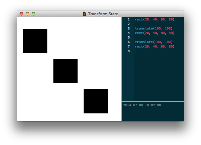
The translate() command shifts the origin relative to the current origin point. Note how calling it repeatedly causes the rectangle – drawn at (20,40) in each instance – to be positioned further and further to the lower right:
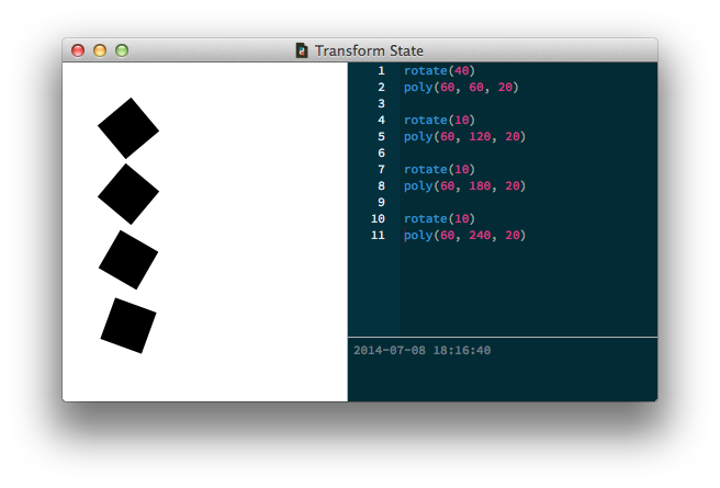
The rotate(), scale(), and skew() commands also work incrementally based on the ‘current’ transformation state. If you first rotate by 40°, all the elements you subsequently draw will be rotated by 40°. If you then rotate by 30°, the current rotation becomes the sum of the two rotations: 40°+30° = 70°.
Likewise, if you keep calling scale(0.8) in your script the
elements on the canvas become smaller and smaller. The second time you call it, the current scale
becomes 0.64 (0.8 × 0.8), the third time it becomes 0.512 (0.64 × 0.8), and so on.
The reset() command undoes any transformation changes from earlier in the script and repositions the origin at the canvas’s top left corner.
Corner mode transformations
We haven’t discussed the transform() command
yet. As you may have already read in the reference you can switch it between two ‘modes’: CENTER and CORNER.
Centered transformation means that all shapes, paths, text and images will rotate, scale, and skew
around their own center (as we would probably expect them to). Using corner-mode transformations means
that elements transform around the current origin point. This can be a difficult concept
to grasp.
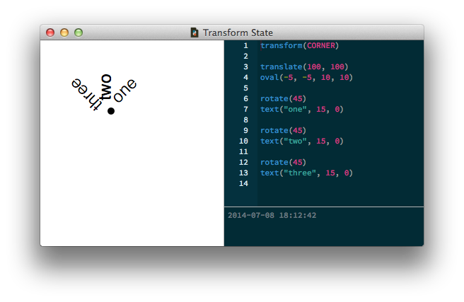
In the example below, we move the origin point to (100,100) and have three pieces of text rotate around it. Without the corner mode transform, they would rotate around their own center and it would be a lot more difficult to position them. Since the corner mode rotation is relative to the origin, we can draw each piece of text at the same relative coordinates (15, 0):
Nested State
In addition to allowing you to change the mode, the transform() command has special ‘clean up’ behavior when used as part of a with block. It allows you to safely create state-in-a-state.
Inside the indentated block, any translate(), rotate(), scale() and skew() commands are valid only until the end of the block. Then the transformation state reverts to how things were prior to the with-statement. This way you can transform groups of elements that need to stay together.
Here’s a short example. Notice that the last rectangle isn’t rotated? That’s because the rotate() call happens within the transform() block and is reset after drawing the second rectangle.

rect(20, 20, 40, 40)
with transform():
    rotate(45)
    rect(120, 20, 40, 40)
rect(220, 20, 40, 40)
You can think of these nested states as analogous to the orbits of planets and moons in our solar system. The planets orbit a central origin point, the Sun, while the moons orbit around their respective planets. You can think of a transform() block as a shift in perspective – you’re setting a new ‘local’ origin point centered not on the Sun but on a particular planet. The planet’s moons orbit this new, local origin (wherever this is), blissfully unaware of the massive star at the center of it all.
size(450, 450)
speed(30)

def draw():
    stroke(0)
    transform(CORNER)

    # This is the starting origin point (the heart of the Sun)
    translate(225, 225)
    arc(0,0, 5)
    text("sun", 10,0)

    for i in range(3):

        # Each planet acts as a local origin for the orbiting moon.
        # Comment out the transform() statement and see what happens.
        with transform():

            # This is a line with a length of 120,
            # that starts at the sun and has an angle of i * 120.
            rotate(FRAME+i*120)
            line(0,0, 120,0)

            # Move the origin to the end of the line.
            translate(120, 0)
            arc(0,0, 5)
            text("planet", 10, 0)

            # Keep rotating around the local planet.
            rotate(FRAME*6)
            line(0, 0, 30, 0)
            text("moon", 32, 0)

        # The origin moves back to the sun at the end of the block.
Point Geometry
PlotDevice scripts are rife with x/y coordinate pairs. You use coordinates to place primitives on the canvas, add line segments to a Bezier, and so forth. Most of the time you can choose these locations through intuition or trial and error. But occasionally you’ll want to perform calculations on points to assemble your compositions in a relative manner.
Sometimes you’ll be working with a pair of points and want to know the angle or distance between them. In other cases you may have a single point and need to calculate a second position relative to the first. To aid in these kinds of tasks, PlotDevice provides a simple class called Point.
Point Objects
You can create a Point by passing a pair of coordinate values to the constructor function and access its coordinates through the x and y attributes.
pt = Point(13,37)
print(pt.y)
>>> 37
You can unpack it back into a pair of values through simple assignment:
x, y = pt
print(x, y)
>>> 13 37
Point objects support basic arithmetic operators (as does the similar Size object):
pt = Point(10, 20)
print(pt * 2)        # Point(20, 40)
print(pt / 2)        # Point(5, 10)
print(pt + 5)        # Point(15, 25)
print(pt + (40, 30)) # Point(50, 50)
pt = Point(10, 20)
sz = Size(200,200)
print(pt + sz)       # Point(210, 220)
print(pt + sz/2)     # Point(110, 120)
Drawing with computed points
Once you have a Point, you can ‘ask’ it all sorts of questions about how it relates to other points with a few useful (and speed-optimized) math methods. You can pull off some neat graphical tricks by combining the Point methods in your scripts.
Finding the angle from a central origin to a randomly positioned point:
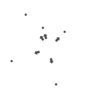
r = 2.0
origin = Point(WIDTH/2, HEIGHT/2)

for i in range(5):
    pt = Point(random(WIDTH), random(HEIGHT))
    arc(pt, r)

    a = origin.angle(pt)
    with transform(CORNER):
        translate(origin.x, origin.y)
        rotate(-a)
        arrow(30, 0, 10)
Orbiting around an origin point:
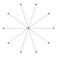
r = 2.0
origin = Point(WIDTH/2, HEIGHT/2)
arc(origin, r) # a.k.a. arc(origin.x, origin.y, r)

for i in range(10):
    a = 36*i
    pt = origin.coordinates(85, a)
    arc(pt, r)
    line(origin, pt)
Drawing perpendicular lines around a circular path:
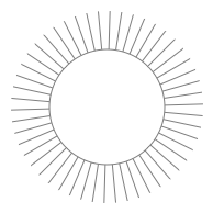
stroke(0.5) and nofill()
path = oval(45, 45, 105, 105)
for t in range(50):
    curve = path.point(t/50.0)
    a = curve.angle(curve.ctrl2)
    with transform(CORNER):
        translate(curve.x, curve.y)
        rotate(-a+90) # rotate by 90°
        line(0, 0, 35, 0)
Angle measurements
As you may remember from trigonometry, there are two commonly used systems for expressing the size of angles. In day-to-day life we’re most likely to encounter ‘degrees’ ranging from 0 to 360. In mathematics it’s more traditional to use ‘radians’ ranging from 0 to 2π. PlotDevice recognizes that different situations may call for different angle units and provides some utilities to make switching between them easy.
A number of commands take an angle as one of the arguments. By default, you’re expected to use degrees. But by calling the geometry() command with DEGREES, RADIANS, or PERCENT you can switch between modes on the fly.
Any subsequent call to a drawing or transformation command that deals with angles will then deal in the newly-specified units. The angle() and coordinates() methods discussed above also obey the geometry() setting – both for interpreting arguments and providing return values.
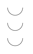
with stroke(0), nofill():
    arc(50,25, 25, range=180)

    geometry(RADIANS)
    arc(50,75, 25, range=pi)

    geometry(PERCENT)
    arc(50,125, 25, range=.5)
To make working with radians more convenient, PlotDevice provides a pair of global constants – pi and tau – representing a half- and full-circle respectively.
Rational Proportions
Sometimes you want to set the position or size of objects in such a way that they interrelate to each other, creating a kind of ‘harmony’ between them. For example, sine waves are great for coordinating motion since they ease in and out.
Another interesting proportional principle is the so-called golden ratio or ‘3-5-8 rule’. It has been around in aesthetics for millennia, though its longevity seems to have as much to do with groupthink as anything ‘fundamental’ about the proportion.
For our purposes, the great thing about it is that it can be expressed as a mathematical series – the Fibonacci sequence.
def fib(n):
    if n == 0: return 0
    if n == 1: return 1
    if n >= 2: return fib(n-1) + fib(n-2)

def goldenratio(n, f=4):
    # Returns two proportional numbers whose sum is n.
    f = max(1, min(f, 10))
    n /= float(fib(f+2))
    return n*fib(f+1), n*fib(f)
Colored rectangles proportioned with the golden ratio:
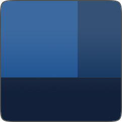
w1, w2 = goldenratio(260)
h1, h2 = goldenratio(260)
b1, b2 = goldenratio(1.0)
b3, b4 = goldenratio(b1)

fill(0, b1/2, b1)
rect(0, 0, w1, h1)

fill(0, b2/2, b2)
rect(w1, 0, w2, h1)

fill(0, b4/2, b4)
rect(0, h1, w1+w2, h2)
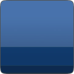
x, y = 0, 0
w, h = 260, 260

th = h # top height
bh = 0 # bottom height
for i in range(10):
    th, bh = goldenratio(th)
    v = float(th)/w + 0.3
    fill(0, v/2, v)
    rect(x, y, w, th)
    y += th
    th = bh
Trigonometry Fundamentals
A sine calculates the vertical distance between two points based on the angle. A cosine calculates the horizontal distance.
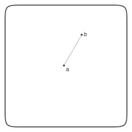
Let’s say we have two points, a and b, connected by a line.
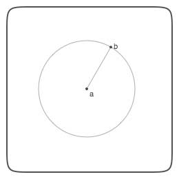
Now let’s assume a is at the origin (or center) of a circle. The circle has a radius equal to the length of the line connecting a and b.
So b is located somewhere on the circle’s circumference.
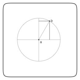
There is a horizontal and vertical distance between a and b.
We can use sine and cosine to determine those distances.
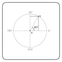
Each line from a to a point on the circle’s circumference (for example, b) has an angle.
Measured counterclockwise, starting from 0°, a circle has a total circumference of 360°. So a line from a going straight up would have an angle of 90°.
In the case of the line between a and b, the angle is 60°.
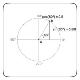
The cosine function calculates the horizontal distance between a and b based on the angle.
The sine function calculates the vertical distance between a and b.
In the case of an angle of 60°, the sine yields 0.5. So the horizontal distance between a and b is half the length of the line between a and b.
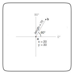
With sine and cosine we can calculate the distance between a and b.
This is useful if we have position coordinates for a and we need to calculate the position of a point b that is orbiting around it.
For 60°, the sine yields 0.5, meaning half the length of the distance between a and b. So the horizontal distance between a and b is 70 × 0.5 or 35.
So b’s x equals a’s x plus 35.
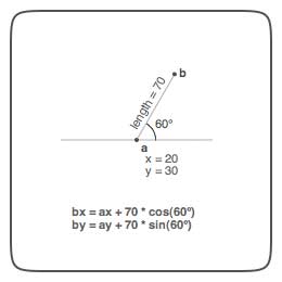
The command in PlotDevice would look like this:
def coordinates(x0, y0, distance, angle):
    from math import radians, sin, cos
    angle = radians(angle)
    x1 = x0 + cos(angle) * distance
    y1 = y0 + sin(angle) * distance
    return x1, y1