Description
In mathematics and computer science, graph theory studies networks of connected nodes and their properties. A graph can be used to visualize related data, or to find the shortest path from one node to another node for example.
Central concepts in graph theory are:
- Node: a block of information in the network.
- Edge: a connection between two nodes (can have a direction and a weight).
- Centrality: determining the relative importance of a node.
- Clustering: partitioning nodes into groups.
The PlotDevice Graph library includes algorithms from NetworkX for betweenness centrality and eigenvector centrality, Connelly Barnes’ implementation of Dijksta shortest paths (here) and the spring layout for JavaScript by Aslak Hellesoy and Dave Hoover (here). The goal of this library is visualization of small graphs (<200 elements), if you need something more robust we recommend using NetworkX.
For those of you looking for the old Graph library built on Boost,
it can still be found here.
Download
| graph.zip (32KB) Last updated for PlotDevice 0.9 Licensed under GPL Author: Tom De Smedt |
Documentation
- How to get the library up and running
- Creating a graph
- Adding nodes and edges
- Retrieving/removing nodes and edges
- Drawing the graph
- Customizing styles and style rules
- Interacting with the animated graph
- Connectivity
- Proximity
- Clustering
- Known issues and limitations
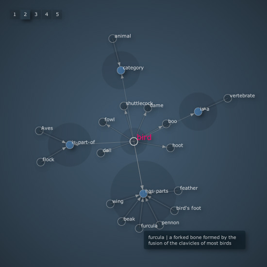
The library has a cool example of a visual browser for WordNet.
How to get the library up and running
Put the graph library folder in the same folder as your script so PlotDevice can find the library. You can also put it in ~/Library/Application Support/PlotDevice/.
graph = ximport("graph")
Outside of PlotDevice you can also just do import graph.
Creating a graph
create(iterations=1000, distance=1.0, layout="spring", depth=True)
The create() command returns a new graph object encompassing the drawing
canvas. The network of connected nodes will originate from the center of the canvas. The
distance parameter controls the spacing between nodes and hence the size of the
graph.
By default, a spring force
layout is used to visualize the graph. Each element in the graph (or node) will
try to get away as far as possible from the others. This is the repulsive force in the
network. At the same time, there are connections (or edges) that keep nodes together.
The greater the weight of an edge the stronger it is in pulling two nodes together. This is the
attractive force in the network. You can also set the layout parameter to
‘circle’ to use a simple circle-based layout.
The forces in the network need to be calculated several times in order for the nodes’ positions to stabilize. The higher the number of iterations the better (but slower) the layout.
| When depth is set to True, the library will attempt to import the PlotDevice Colors library for gradient and shadow effects. |
The returned graph object has the following properties:
- graph.nodes: a list of all the node objects in the graph.
- graph.edges: a list of all the edge objects in the graph.
- graph.leaves: a list of all the nodes with only one connection.
- graph.root: the root node in the graph.
- graph.done: True when the graph’s layout is completely calculated.
- graph.distance: the scale of the graph when drawn (usually a number between 0.5
and 2.0).
- graph.density: a number between 0.0 and 1.0 indicating the number of connections.
- graph.is_sparse: True when there are few connections in the graph (density is 0.35 or less).
- graph.is_dense: True when there are a lot of connections (density is 0.65
or more).
- graph.is_complete: True when all nodes are connected to all other nodes (density is 1.0).
- graph.layout: the layout object used to calculate the graph.
- graph.events: the event object used to monitor mouse dragging and clicking.
- graph.styles: the styles object used to colorize and draw the graph.
Adding nodes and edges
graph.add_node(id, radius=8, style="default", category="", root=False)
graph.add_edge(id1, id2, weight=0.0, length=1.0, label="")
You can add nodes (e.g. blocks of information you want to connect) to the graph with the graph.add_node() method. The id parameter uniquely identifies each node, it will appear as a label on each node once the graph is visualized. When the root parameter is True it will set this node as the graph’s root.
The graph.add_node() method returns a node object with the following properties:
- node.id: the node’s unique id.
- node.r: the node’s radius.
- node.style: the name of the style used to colorize and draw the node.
- node.category: a category this node belongs to.
- node.label: displayed when the node is drawn (by default, its id).
- node.x: the horizontal position of the node on the canvas.
- node.y: the vertical position of the node on the canvas.
- node.links: a list of all node objects connected to this one.
- node.edges: a list of all edge objects this node is involved with.
- node.is_leaf: True when the node has only one connection.
- node.weight: a number between 0.0 and 1.0 reflecting the node’s relevance in the graph.
- node.traffic: a number between 0.0 and 1.0 reflecting the amount of shortest paths.
- node.eigenvalue: identical to node.weight.
- node.betweenness:identical to node.traffic.
We’ll look at the details of a node’s weight and traffic in the section on graph proximity.
You can connect two nodes with the graph.add_edge() method. It takes two node id’s,
an optional weight (ranging between 0.0 and 1.0) and an optional label to display
near the edge when it is drawn.
An edge object is returned. It has the following properties:
- edge.node1: the node object from which the connection originates.
- edge.node2: the node object in which the connection ends.
- edge.weight: the weight or strength of the connection.
- edge.length: the individual length of the edge (1.0 by default).
- edge.label: a label to display near the edge when drawn.
|
|
graph = ximport("graph") g = graph.create(iterations=500, distance=0.8) g.add_node("PlotDevice") g.add_node("Core Image", category="library") g.add_edge("Core Image", "PlotDevice") g.solve() g.draw() |
Retrieving/removing nodes and edges
The graph object has graph.nodes and graph.edges properties that list all of the nodes and connections it contains. It also has a graph.node() and a graph.edge() method that returns nodes and edges based on id’s:
graph.node(id)
graph.edge(id1, id2)
Furthermore, a graph behaves as a dictionary with node id keys linking to node object:
for id in graph:
    print graph[id].style
To remove nodes and edges you can use the methods below. The graph.clear() method removes all nodes and all edges and resets the graph’s layout. This is useful when you want to dynamically reload a graph.
graph.remove_node(id)
graph.remove_edge(id1, id2)
graph.clear()
You can get access to all the nodes connected to a given node from the node.links
list. This list also has a fast node1.links.edge(node2) method that retrieves the edge
between two nodes.
Drawing the graph
Before we can draw the graph to the canvas, we first need to calculate its layout. This may take several seconds or more for graphs with many nodes. More nodes slow down the process, as do more visual elements like edge labels. The following methods are involved:
graph.prune(depth=0)
graph.update(iterations=10)
graph.solve()
graph.draw(weighted=False, directed=False, highlight=[], traffic=None)
The graph.prune() method removes orphaned nodes that have no connections . If depth is 1 it removes nodes that have one ore less connections, and so on. Pruning is often a good idea, as the less nodes there are in a graph the faster the layout is calculated.
The graph.update() method calculates a portion the total iterations. This is useful in an animation when you want the graph to slowly unfold. When the entire layout has been calculated, the graph.done property will be True.
The graph.solve() method does all the iterations at once. If you’re not running an animation you usually use this method before drawing the graph.
The graph.draw() method draws the graph to the canvas. It will originate from the canvas center (although you can nudge it horizontally or vertically with optional dx and dy parameters).
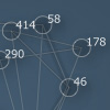
| The optional weighted parameter indicates an edge’s weight by adding a subtle shadow to it when set to True. |
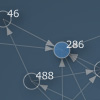
| The optional directed parameters indicates an edge’s direction with an arrow when set to True. |
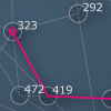
| The optional highlight parameter indicates a path between two nodes. Node id’s in the path are supplied as a list. Usually this is a value returned from the graph.shortest_path() method. |
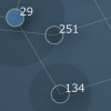
| The optional traffic parameter can be a number, representing the amount of top-trafficked nodes to highlight. Nodes with a high traffic have a lot of shortest paths passing through them therefore have a central role in the network. |
Layout
If you’re using the graph in an animation, you can use the graph.layout.refresh() method to trigger some new iterations. This is useful when you are for example dynamically adding new nodes after the layout has stopped. The graph.layout.reset() restarts the layout from scratch.
graph.layout.refresh()
graph.layout.reset()
When using the spring-force layout, graph.layout has a tweak() method that allows you to play around with the internals of the layout algorithm:
graph.layout.tweak(k=2, m=0.01, w=15, d=0.5, r=15)
The k parameter is the force constant by which nodes are pushed away from each other, m is a dampener for the total attractive/repulsive force, w is a weight multiplier (so heavier edges have a bigger attraction), d is the maximum node movement per iterations and r is the radius of repulsive force originating from each node.
You may find the following layout properties easier to use:
- graph.layout.force: the attractive/repulsive force in the layout (0.01 by default).
- graph.layout.repulsion: the repulsive radius originating from each node (15 by default).
If you are using the circle layout, graph.layout has only one property:
- graph.layout.orbits: the number of circles used in the layout (2 by default).
Customizing styles and style rules
You can customize the look and feel of the graph down to the bottom. The graph.styles dictionary has different styles for different nodes. Each style has some color and font properties and a range of methods for drawing each element in the graph. The styles dictionary is accompanied by a styleguide containing rules that define how and when to apply the styles. You can easily modify existing styles, create new ones, and devise your own rules for how to apply them.
Predefined styles
Let’s have a look at the different styles in a graph:
| default: this style is used for nodes that have no style defined. Edges will always use the default stroke color. | |
| light: a style with subtly highlighted nodes. By default it is used for nodes directly connected to the root. | |
| back: a style with green colored nodes and curved edges. By default it is used to indicate a previous root node (e.g. like a back button). | |
| marked: a style that marks nodes with a dot. By default it is used to indicate peers of the root node. | |
| dark: a style with blue colored nodes. By default it is used to indicate nodes with four or more connections. | |
| important: a style with big blue colored nodes that get an extra outline. By default it is used for nodes that have a weight of 0.75 or more. | |
| highlight: a style that marks paths in pink. By default it is used to indicate the highlight path supplied to graph.draw(). | |
| root: a style that marks the root node in the graph. |
print graph.styles.keys()
>>> ['default', 'light', 'back', 'marked', 'dark',
>>>  'important', 'highlight', 'root']
You can change the properties of each of the individual style objects:
graph.styles.root.fontsize = 20
Or set a property on all styles:
graph.styles.stroke = color(1)
Here’s an example of how to add your own custom style:
s = g.styles.create("red")
s.fill = color(1, 0, 0.25, 0.75)
Style properties
A style object has the following properties:
- style.background: graph background color (always picked from the default style).
- style.fill: fill color for nodes. The default fill is also used as backdrop on weighted edges.
- style.stroke: the stroke color for node outlines. The default stroke is used for all edges.
- style.strokewidth: the width of node outlines and edges.
- style.text: text color used for node and edge labels.
- style.font: font used for node and edge labels.
- style.fontsize: fontsize for node and edge labels.
- style.textwidth: if the label ’s width exceeds this number it gets wrapped to the next line.
- style.align: aligns the node label either RIGHT or CENTER.
- style.depth: True when this style uses the Colors library to render dropshadows.
Styleguide
You can assign the name of a style to node.style and then when the network is drawn the node will be visualized using the style’s properties and drawing methods.
You can assign styles by hand - for example, here’s how to make all nodes with a weight of more than 0.6 ‘important’:
for node in graph.nodes:
    if node.weight > 0.6:
        node.style = "important"
Rules like these (’heavy nodes are important’) can also be bundled in the styleguide dictionary:
graph.styles.guide.append("important", lambda graph, node: node.weight > 0.6)
The default rules in the guide are:
{ "light"     : lambda graph, node: graph.root in node.links
  "dark"      : lambda graph, node: len(node.links) > 4
  "important" : lambda graph, node: node.weight > 0.75
  "root"      : lambda graph, node: node == graph.root
  "back"      : lambda graph, node: node == graph.events.clicked
}
- nodes directly connected to the root get the light-style
- nodes with four or more connections get the dark-style
- nodes with a weight greater than 0.75 get the important-style
- the root node gets the root-style
- the node that was last clicked gets the back-style
Below is another interesting rule that keeps clusters of nodes together. The edges of nodes
that have only one connection become shorter, all others become longer. The default styleguide
uses a simpler version.
def cluster(graph, node):
    if node == graph.nodes[0]:
        for e in graph.edges: e.length = 4.0
    if len(node.links) == 1:
        graph.edge(node.id, node.links[0].id).length = 0.2

graph.styles.guide.append("cluster", cluster)
To apply the styling rules to the network:
graph.styles.apply()
There’s a graph.styles.guide.order property (which is a list of style names) that defines the sequence in which style rules will be applied. There’s also a graph.styles.clear() method to remove all the rules.
Style drawing methods
A style has customizable drawing methods. We will only go into this briefly here. Developers can check the source code in the style.py file in the library. Here’s a quick example of how we add our own custom patch for edges:
|
|
def curly_edge(style, path, edge, alpha=1.0): path.moveto(edge.node1.x, edge.node1.y) path.curveto( edge.node1.x - 40, edge.node1.y, edge.node2.x + 40, edge.node2.y, edge.node2.x, edge.node2.y, ) graph.styles.default.edge = curly_edge graph.draw() |
Interacting with the animated graph
You can use very small graphs (<100 nodes) in an animation and watch them unfold fluidly. The graph object has functionality for mouse interaction as well, bundled in the graph.events object. It has the following properties:
- graph.events.hovered: None or the node over which the mouse hovers.
- graph.events.pressed: None or the node on which the mouse is pressing down.
- graph.events.dragged: None or the node being dragged.
- graph.events.clicked: None or the last node clicked.
- graph.events.popup: when True, will display a popup window over the hovered node.
|
|
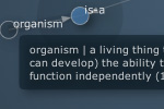
When you hover over a node the graph.events.hover() method fires. It will try to display a description of the node’s id from WordNet (if you have the Linguistics or WordNet library installed). To display your own popup text for a given node, register it in the graph.events.popup_text dictionary: graph.events.popup_text["organism"] = "hello" In an animation you can also simply press down on a node and drag it around to where you want it. The graph will stabilize by itself. Last but not least, if you click on a node graph.events.click() will fire. This method takes one node parameter and does nothing by default, so if you want clicking behavior you’ll have to assign your own command: def click(node): print node.id+" clicked" graph.events.click = click |
Connectivity
Finding out if two nodes are connected (with zero or more other nodes in between them) is
easy enough with the node.can_reach() method, which returns either True or
False:
node.can_reach(node, traversable: lambda node, edge: True)
What is intriguing about this method is the optional traversable parameter. You can pass it a custom command. This command takes two parameters, a node and an edge, and returns True if the given node is allowed to travel over the given edge.
This allows for more elaborate searches. For example, in the Perception library all edges have a type, like is-part-of or is-related-to. Traversables are used to check if two nodes are connected using only specific types of edges: an oak is a tree only if the oak node can reach the tree node using only is-a edges (and not, for example, is-property-of).
Proximity
Graphs are not only useful to visualize data, but to analyze it as well. Knowing what the shortest path is, how to get from one node to another, can tell us something of how those nodes relate to each other.
Dijkstra’s shortest path algorithm is a way to find the closest route from one node to another in the network. For example, if the nodes in the network represent cities and their strength represent driving distances between pairs of cities connected by a direct road, Dijkstra’s algorithm can be used to find the shortest route between two cities.
graph.shortest_path(id1, id2, heuristic=None, directed=False)
The graph.shortest_path() method returns a list of node id’s connecting the two nodes with the given id’s. If no connection can be found it will return None.
path = graph.shortest_path(119, 381)
graph.draw(highlight=path, weighted=True)
print path
>>> [119, 383, 478, 78, 381]
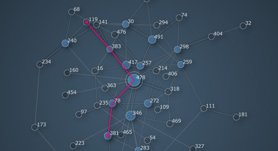
When searching for a shortest route the edge weight becomes important. Edges with a higher weight represent shorter routes. You can think of an edge with a weight of 1.0 as a highway and an edge with a weight of 0.0 as a mountain trail. So even if an edge looks longer onscreen (because it yields a nicer layout for example) it might still be a better candidate to travel by. Likewise, a straight connection may be abandoned in favor of a detour on heavier edges.
Optionally you can also supply your own heuristic function to tweak the pathfinder. It is
a command that takes two node id’s as its parameters and returns a number (usually between -1
and +1). The lower this number gets the more interesting the connection between the two
nodes becomes. For example, in a game environment you could use edge weight to represent the
quality of a road through the world, and supply heuristic terrain penalties for mountains,
swamps, oceans - to discourage AI-controlled characters from trying to cross the ocean or walk
through walls to reach an enemy.
Centrality
How a node is connected to other nodes influences its importance in the network. The Graph library uses two measurements to determine a node’s importance: betweenness centrality and eigenvector centrality.
- Betweenness centrality: nodes that occur on many shortest paths have a higher
betweenness. You can think of such nodes as being hubs, landmarks, city centers and so on.
The betweenness centrality of a node is represented in the node.traffic property as a
number between 0.0 and 1.0.
- Eigenvector centrality: nodes that (indirectly) connect to high-scoring nodes get a better score themselves. In this case the edge direction plays an important role. Ideally, everyone is pointing at you and you are pointing at no-one - meaning you are at the top of hierarchy. The eigenvector centrality is represented in the node.weight property as a number between 0.0 and 1.0.
|
|
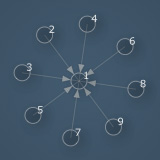
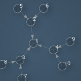
Consider a node that has eight connections to other nodes. Consider another node that has three connections that each connect to two other nodes. An initial naive estimate would be to say that the node in the first case is more important because it has eight connections. However, the node in the second case has the potential to influence up to nine other nodes, and therefore it has a higher importance in the network. The king of a country has only his advisors as direct connections, but his influence is obviously much higher than a post office secretary in the same country who may have hundreds of direct connections with his clients. Eigenvalue centrality is what Google’s PageRank algorithm uses to rank web pages. Read some more interesting details on the 20bits blog. |
The graph has two methods that return a list of nodes sorted according to traffic or weight:
graph.nodes_by_traffic(threshold=0.0)
graph.nodes_by_weight(threshold=0.0)
If you dynamically add new nodes to the graph the balance can shift and you may want to recalculate the proximity values:
graph.betweenness_centrality(directed=False)
graph.eigenvector_centrality(reversed=True, rating={},
                             start=None, iterations=100, tolerance=0.0001)
Both methods recalculate a node’s traffic/weight property and return a dictionary of node id’s linked to a value between 0.0 and 1.0. You may also notice the optional rating parameter which is a dictionary of node id’s linked to a score to influence it’s weight (e.g. Google not only examines a web page’s connections but also its contents - the score of a page’s content could be reflected in the ranking dictionary).
Clustering
Clustering means the classification of objects into different groups, so that all the objects in a group share some common traits (e.g. a rabbit and a bird both belong to the animal group). Clustering is in part related to how you organize your graph, and in part to what analysis you can then perform on the graph. The Graph library has some simple tools for cluster analysis.
graph.nodes_by_category(name)
The graph.nodes_by_category() method returns a list of all nodes that have their category property equal to the given name.
graph.fringe(depth=2)
The graph.fringe() method returns a list of nodes on the perimeter of the graph. With a depth of 1 it returns all the leaf nodes, with a depth of 2 all the leaf nodes and nodes connected to leaf nodes, etc.
graph.sub(id, distance=1)
The graph.sub() method returns a new graph object that is a subset of the
given graph. If distance is 0, it will contain only the node with the given id.
If distance is 1, it will contain the node and all nodes directly connected to that node. If
distance is 2, it will also contain all nodes that are connected to nodes directly
connected to the given node, and so on. You can also supply a list of id’s instead of a single
id.
Yet another way to create a subgraph is to pass a filtering function instead of an id. For example:
graph =  ximport("graph")
g = graph.create(iterations=500, distance=0.8)

g.add_node("PlotDevice")
g.add_node("Linguistics", category="library")
g.add_node("WordNet", category="library")

g.add_edge("Linguistics", "PlotDevice", label="related-to")
g.add_edge("WordNet", "PlotDevice", label="related-to")
g.add_edge("WordNet", "Linguistics", label="part-of")

# subgraph containing only library nodes:
g = g.sub(lambda node: node.category == "library", distance=0)
g.distance = 1.4
g.solve()
g.draw(directed=True)

Note: remember that if you want to draw a subgraph, you need to recalculate the layout with the update() or solve() method.
Subgraph set theory
Set theory deals with union, difference and intersection operations between sets of elements. You can compare subgraphs to find out which nodes they have in common (intersection), which nodes they do not have in common (difference) or which is the combined set of both subgraphs (union).
- Union: all elements from A and all elements from B.
- Difference: elements that appear in A but not in B.
- Intersection: elements that appear in A as well as in B.
The following methods will return a new subgraph based on set operations:
graph1.join(graph2) # union, graph1 | graph2 also works
graph1.subtract(graph2) # difference, graph1 - graph2 also works
graph1.intersect(graph2) # intersection, graph1 & graphs2 also works
Cliques
In graph theory, a clique is a graph in which each node is connected to all the other nodes. There’s a graph.is_clique property that returns True when the graph is complete. Since each node is connected to every other node in a complete graph, its density will be 1.0.
graph.clique(id, distance=0)
graph.cliques(id, threshold=3, distance=0)
The graph.clique() method returns a subgraph of the biggest clique around the node with the given id. It takes an optional distance parameter which will also include other nodes connected to the nodes in the clique (see the distance parameter for the graph.sub() method).
The graph.cliques() method returns a list of subgraphs that are cliques of at least threshold nodes.
Partitioning
Finally, there’s a powerful technique to split a graph into its unconnected subgraphs. Sometimes your graph may contain two or more clusters of nodes without connections between them (especially if you don’t know where the data came from). The graph.split() method will return a list of unconnected subgraphs, sorted biggest-first:
subgraphs = graph.split()
subgraphs[0].solve()
subgraphs[0].draw()
Known issues and limitations
Exporting a graph as a PDF may crash PlotDevice on some systems.
Disabling dropshadow and gradient effects should remedy this:
g = graph.create(depth=False)
